Charts
rich_ext::chart draws data with text:
Sparkline: one line, one cell per value.BarChart: a label, a bar and a value per row; groups of bars side by side or stacked.Histogram: raw values counted into bins, drawn as bars.LineChart: one or more series as lines or scattered points, with axes and a legend.PieChart: shares of a whole as slices of a disc or a donut, with a legend of percentages (below).
And the pieces of a dashboard:
GaugeandBulletChart: a value against a range, with a target and threshold bands, on one line or the full width.Heatmap: a labelled grid of values drawn as shades, with a legend.StatusMatrix: rows and columns of states (pass, fail, skip, flaky or your own), each a symbol and a colour.KpiCard: a label, a value, its change, a sparkline and a status.Timeline: labelled ranges on a numeric or seconds scale, overlaps stacked, with milestones; a Gantt strip when every range has its own row.
And for comparing (below):
DistributionandDistributionSet: the count, quantiles and mean of a set of values, with a box-and-whisker strip on one line; several stacked on one scale.SmallMultiples: a grid of titled charts on one value scale, fitted to the width.
Every chart also says what it shows in words, for a screen reader (accessible text).
And laid out as ratatui's widgets, so a ported app looks the same (below):
Chart: datasets on two axes, as lines, points, bars or areas, the areas stacked if asked.Canvas: shapes, text and a world map in world coordinates.FillGaugeandLineGauge: ratatui'sGaugeandLineGauge.
Each chart is a renderable. It measures itself, so it works in a Table
cell, a Panel or a Live display. It never writes a line wider than the
width it is given: when space is short it drops labels, values and axes
before it drops data.
A Chart, a Canvas, a vertical BarChart, a Sparkline and a
FillGauge also fill the height they are given, as ratatui's widgets
fill their area: a Layout region, a Panel with a height, or an
intuiTUIve node through
renderable(move || chart(..)). Their own height (.height(n),
.rows(n), .bar_width(n)) wins; printed on their own, with no height
given, they keep their defaults.
The examples come from
guide_charts.rs,
and the pies, stacked charts, QR codes and gradients from
guide_charts_extra.rs.
The module needs no feature (QR codes need qr):
cargo run -p rs-rich-ext --example guide_charts
cargo run -p rs-rich-ext --example charts            # every chart on one screen
cargo run -p rs-rich-ext --example charts -- --ascii
cargo run -p rs-rich-ext --example kpi_dashboard     # cards, a matrix and a timeline, live
cargo run -p rs-rich-ext --example guide_charts_extra --features qr
The styles are theme keys (chart.*). Pass rich_ext::extended_theme() to
the console builder to get them, or define them in your own theme. Without
them the same defaults are used.
The same charts are in Python as rs_rich.chart,
and in the shell as rich chart.
Sparklines
Sparkline::new(values) draws each value as a cell whose height shows where
it falls between the smallest and largest value:
fn show_sparklines(console: &Console) {
    console.print(&Sparkline::new(REQUESTS));
    // Name the extremes and count the values over a threshold.
    console.print(&Sparkline::new(REQUESTS).min_max(true).threshold(40.0));
    // Two values per cell.
    console.print(&Sparkline::new(REQUESTS).charset(Charset::Braille));
    // Fewer cells than values: each cell is the mean of its bucket.
    let narrow = Console::builder().width(8).color_system(None).build();
    console.print(&Text::new(
        narrow.render_to_string(&Sparkline::new(REQUESTS)),
    ));
}

- It is one cell per value wide. Given fewer cells, it resamples: the values are split into as many equal buckets as there are cells, and each cell shows the mean of its bucket's values.
.min_max(true)styles the lowest and highest cell (chart.min,chart.max) and writesmin 12 max 52after the line..threshold(40.0)styles the cells above 40 withchart.overand writes4 > 40(four values are above it).- The words are what make the extremes and the threshold readable without colour. They are the first thing left out when the line does not fit.
.range(min, max),.min(v)and.max(v)fix the scale; values outside it are clamped. NaN and infinite values are gaps.
Taller, backwards, with gaps
What ratatui's Sparkline has, and more rows than one:
fn show_ratatui_sparklines(console: &Console) {
    let wave: Vec<f64> = (0..48).map(|i| (i as f64 / 4.0).sin() * 10.0).collect();
    // Three rows tall, eight heights a row.
    console.print(&Sparkline::new(wave.clone()).rows(3));
    // Right to left, with gaps drawn and one value styled.
    let gaps = wave
        .iter()
        .enumerate()
        .map(|(i, v)| (i % 9 != 4).then_some(*v));
    let mut styles = vec![None; 48];
    styles[12] = Some("bold yellow".to_string());
    console.print(
        &Sparkline::optional(gaps)
            .rows(2)
            .direction(Direction::RightToLeft)
            .absent("░", "red")
            .styles(styles),
    );
    // Braille over two rows: two values a cell.
    console.print(&Sparkline::new(wave).rows(2).charset(Charset::Braille));
}
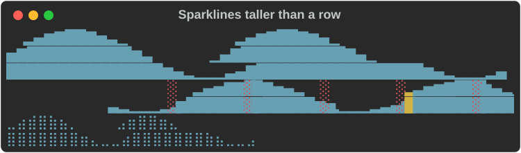
.rows(n)makes itnrows tall, eight heights a row in blocks and four in Braille. Without it, it fills the height it is given..direction(Direction::RightToLeft)puts the first value at the right edge, and the summary before the bars.Sparkline::optional(values)takesOption<f64>s: eachNoneis a gap..absent(symbol, style)draws gaps with a symbol down the whole column, as ratatui'sabsent_value_symbol..styles(vec![..])gives each value a style of its own; it wins over the marks of.min_maxand.threshold..levels(Levels::Three)draws with ratatui's three-level set (▄█), for fonts without the eighths.
Bars
BarChart draws a row per bar: the label, the bar and the value.
fn show_bars(console: &Console) {
    let chart = BarChart::new()
        .bar("api", 412.0)
        .bar("web", 268.5)
        .bar("worker", 97.0)
        .push(Bar::new("cron", 12.0).style("chart.over"))
        .bar_width(30);
    console.print(&chart);
    // Negative values extend left of zero.
    console.print(
        &BarChart::from_pairs([
            ("north", 18.0),
            ("south", -7.5),
            ("east", 4.0),
            ("west", -12.0),
        ])
        .bar_width(30),
    );
}
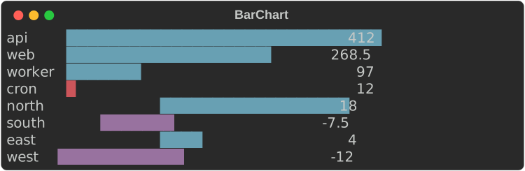
- Bars are measured from zero. The scale runs from the smallest to the
largest value and always includes zero;
.max(100.0)or.range(..)fix it. - Blocks give eighth-cell precision (
█▉▊▋▌▍▎▏). A value above zero always shows at least a sliver. - Negative values extend left of zero, at whole-cell precision, in
chart.negative. The written value keeps its minus sign, so the chart reads the same without colour. Bar::new(label, value).style(..)styles one bar;.style(..)on the chart styles them all. Both take a theme key or a style definition.- The bar is 40 cells by default (
.bar_width(n)). When the width is short the bar shrinks to 4 cells, then the values go, then the labels are cut with…. .show_values(false)leaves the values out;.format(ValueFormat::Fixed(1))writes them with one decimal instead of the compact form (1.2k,3.4M).
Vertical bars
.orientation(Orientation::Vertical) stands the bars up side by side, with
the labels underneath:
fn show_vertical(console: &Console) {
    let week = BarChart::from_pairs([
        ("mon", 31.0),
        ("tue", 42.5),
        ("wed", 38.0),
        ("thu", 51.0),
        ("fri", 47.0),
        ("sat", 12.0),
        ("sun", 9.5),
    ])
    .orientation(Orientation::Vertical)
    .bar_width(8);
    console.print(&week);
    // Negative values hang below zero, their values under them.
    console.print(
        &BarChart::from_pairs([("q1", 18.0), ("q2", -7.5), ("q3", 4.0), ("q4", -12.0)])
            .orientation(Orientation::Vertical)
            .bar_width(6),
    );
}
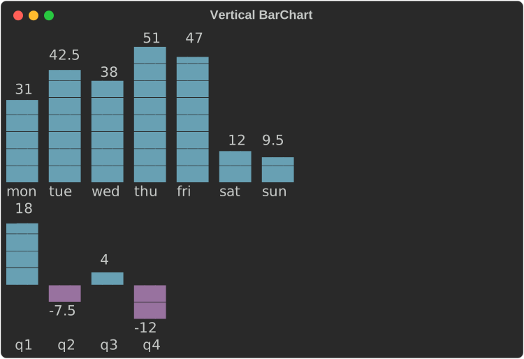
.bar_width(rows)is the tallest bar's height here, 8 rows by default.- Blocks give eighth-row precision (
▁▂▃▄▅▆▇█), Braille half rows (⣤⣿), ASCII#and a half.. A value above zero always shows at least a sliver. - Each bar gets a slot as wide as the widest label or value, with a cell between slots, and is up to 3 cells thick. Each value sits just above its bar.
- Negative values hang below the zero line at whole-row precision, their values under them.
- When the width is short the values go first, then the labels are cut (and left out below two cells), then the gaps between bars. Bars that still do not fit are left off the right.
- An explicit
.thickness(n),.bar_gap(n)or.group_gap(n)is kept, as ratatui keeps them: the slots narrow to the thickness, then as many whole bars as fit (with their gaps) are drawn, from the first, and the rest are left off. 24 bars 3 cells thick and 2 apart show the first 8 in 40 cells. - Without
.bar_width(..)a vertical chart fills the height it is given, less its labels and values. Histogramtakes.orientation(..)too.
Groups, text values and styles
What ratatui's BarChart has, by this crate's names:
fn show_ratatui_bars(console: &Console) {
    // Revenue by month for three companies: groups, text values on the
    // bars, four cells thick.
    let mut chart = BarChart::new()
        .orientation(Orientation::Vertical)
        .thickness(4)
        .bar_gap(1)
        .group_gap(2)
        .values_inside(true)
        .bar_width(6);
    for (month, values) in [("Jan", [8.5, 6.5, 7.0]), ("Feb", [9.0, 7.5, 8.5])] {
        let mut group = BarGroup::new(month);
        for (name, value, colour) in [
            ("BITE", values[0], "blue"),
            ("TART", values[1], "white"),
            ("BAKE", values[2], "bright_red"),
        ] {
            group = group.bar(
                Bar::new(name, value)
                    .text(format!("{value:.1}M"))
                    .style(colour)
                    .value_style(format!("black on {colour}")),
            );
        }
        chart = chart.group(group);
    }
    console.print(&chart);
    // The seasons, their ranges written along the bars.
    let seasons = BarChart::new()
        .push(Bar::new("", 51.0).text("Winter 37-51"))
        .push(Bar::new("", 65.0).text("Spring 40-65"))
        .push(Bar::new("", 77.0).text("Summer 54-77"))
        .push(Bar::new("", 71.0).text("Fall 41-71").value_style("bold"))
        .bar_gap(1)
        .style("#203060")
        .value_style("grey70 on #203060")
        .values_inside(true)
        .bar_width(30);
    console.print(&seasons);
}
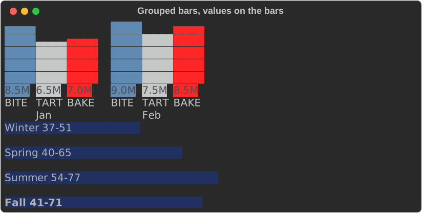
.group(BarGroup::new("Jan").bar(..))adds bars with a label: centred under the group when vertical, on the row after it when horizontal..group_gap(n)sets them apart (1 cell, or 2 rows, by default)..thickness(n)is ratatui'sbar_width: how many cells wide a vertical bar is, or rows tall a horizontal one (a horizontal bar's label and value sit on its middle row)..bar_width(n)keeps its meaning here: the longest bar's length, or the tallest column's height..bar_gap(n)is the space between bars: 1 cell vertical, no rows horizontal, by default.Bar::new(..).text("76°")writes text instead of the value..label_style(..)and.value_style(..)style the labels and values, and a bar's own.label_style(..)and.value_style(..)go over them..values_inside(true)writes each value on its bar, as ratatui does: from the start of a horizontal bar, running on past its end in the bar's colour; on the bottom row of a vertical one, centred and cut to its thickness. Without a value style, a value on its bar is the bar's colour reversed.
Stacked bars
BarGroup::new("Q1").stacked() draws a group as one bar, its bars end to
end, labelled with the group's label and its total written after it (above
it, vertical):
fn quarters() -> BarChart {
    let quarter = |label: &str, api: f64, web: f64, cron: f64| {
        BarGroup::new(label).stacked().bars([
            Bar::new("api", api),
            Bar::new("web", web),
            Bar::new("cron", cron),
        ])
    };
    BarChart::new()
        .group(quarter("Q1", 41.0, 26.0, 8.0))
        .group(quarter("Q2", 38.0, 31.0, 11.0))
        .group(quarter("Q3", 52.0, 24.0, 9.5))
        .group(quarter("Q4", 47.0, 35.0, 14.0))
}

fn show_stacked(console: &Console) {
    console.print(&quarters().bar_width(40));
    console.print(&quarters().orientation(Orientation::Vertical).bar_width(8));
}
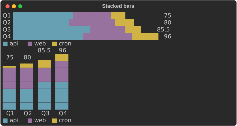
- Each part takes
chart.series.Nby its place in the stack (or its ownBar::style), and the legend under the chart names the parts after the first stack's bars..legend(false)hides it. - Without colour each part has its own fill:
█▓░▒in blocks,⣿⣤⠿⠶in Braille,#=+:in ASCII, and the legend shows the fills:
- Parts above zero stack up from zero, parts below it down from zero; the scale fits both sums. Part edges fall on whole cells; with colour the last part ends in a partial cell, as a plain bar does.
- Other bars in the same chart are stacks of one.
.values_inside(true)has no effect on stacks: their totals are written outside. - The accessible text names each stack's total and parts:
Stacked bar chart, 2 stacks of 2 parts, totals at 6, thenQ1 total 6 (a 4, b 2), Q2 total 6 (a 3, b 3).
Histograms
Histogram::new(values).bins(n) counts raw values into n bins of equal
width and draws them as a BarChart:
fn show_histogram(console: &Console) {
    console.print(&Histogram::new(latencies()).bins(8).bar_width(30));
}
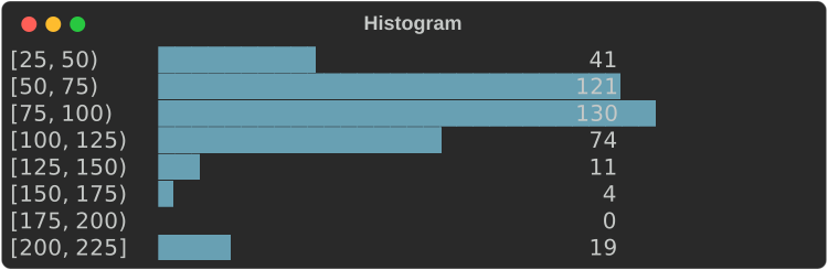
- Each label is
[low, high), and the last[low, high], so every value falls in exactly one bin, the one its label names: a value on an edge counts in the bin that edge starts. - The edges are written exactly, never rounded: when the compact form would
round one (
1250as1.2k), they are all written in full ([1000, 1250))..edges()returns them without floating-point noise (0.3, not0.30000000000000004). - Without
.range(min, max), the bin width is rounded up to 1, 2, 2.5 or 5 times a power of ten and the first edge down to a multiple of it, so the labels are round numbers. The last bins may then be empty. - With
.range(min, max)the bins split that range exactly, and values outside it are not counted. NaN and infinite values are never counted. .counts()and.edges()return the numbers;.to_bar_chart()the chart.
Pie and donut charts
A PieChart draws shares of a whole as slices of a disc, clockwise from
the top, with a legend of labels and percentages beside it (under it when
there is no room):
fn traffic() -> PieChart {
    PieChart::from_pairs([
        ("api", 412.0),
        ("web", 268.5),
        ("worker", 97.0),
        ("cron", 12.0),
    ])
}

fn show_pie(console: &Console) {
    console.print(&traffic());
    // A ring, with the total in the hole, and the values in the legend.
    console.print(
        &traffic()
            .donut(0.5)
            .centre_text("790")
            .show_values(true)
            .height(10),
    );
    // In words, for a screen reader.
    console.print(&Text::new(traffic().accessible_text(80)));
}
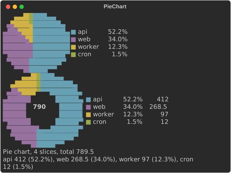
- Half blocks by default: two pixels a cell (
▀▄█), each slice in itschart.series.Ncolour (orSlice::new(..).style(..)), so two slices can share a cell and the disc is round at twice the resolution. - Without colour each slice is drawn a cell at a time in its own fill
(
█░▓▒▚▞), and the legend shows the fills.Charset::Brailledraws 2×4 dots a cell and leaves out the dots on the edges between slices, so the wedges read without colour too.Charset::Asciifills with#+@:%=o*:
.donut(0.5)cuts a hole half the radius;.centre_text("790")writes in it when it fits..height(n)sets the disc's rows (it is twice as wide); otherwise it fills the height it is given, or takes 8 rows. Given less width, the disc shrinks..show_percentages(false)and.show_values(true)choose the legend's columns;.legend(false)hides it.- A value that is not a finite number above zero takes no part of the disc
and its percentage is written
-; a slice too small for a cell is still in the legend and the accessible text (Pie chart, 4 slices, total 789.5, then each slice's value and share).
Line and scatter charts
A LineChart plots one or more Series. Series::line(name, points) joins
its points, Series::scatter(name, points) does not, and
Series::from_values(name, values) puts the values at x = 0, 1, 2, …
let cpu = (0..60).map(|i| (i as f64, 50.0 + 30.0 * (i as f64 / 8.0).sin()));
let memory = (0..60).map(|i| (i as f64, 30.0 + i as f64 * 0.8));
let alerts = [(7.0, 92.0), (23.0, 88.0), (41.0, 95.0), (55.0, 90.0)];
LineChart::new()
    .series(Series::line("cpu %", cpu))
    .series(Series::line("memory %", memory))
    .series(Series::scatter("alerts", alerts))
    .y_range(0.0, 100.0)
    .height(11)
    .width(64)
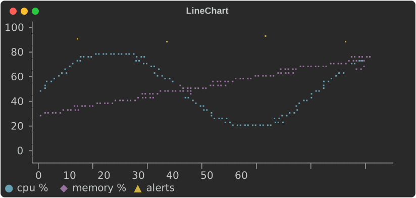
- The plot is Braille by default: each cell holds 2×4 dots, so a chart 60 cells wide has 120 points across.
- Every row and column of the plot stands for one exact value, at its centre. Axis labels sit on evenly spaced rows and columns, and each label is the value of the row or column it is on; nothing is rounded to fit.
- Without
.y_range(..)and.x_range(..), each scale rounds out to a step of 1, 2, 2.5 or 5 times a power of ten that falls on whole rows or columns. The x scale may then run a little past the last point. - When the compact format cannot write those round values exactly, as with
years (
2015would read2.0k) or millisecond timestamps, the labels are all written in full (2015,2016, …) rather than spreading the data thinly over a coarser, writable step. - With a fixed range, a row or column gets a label only when the format
writes its value exactly, so a range must divide into the rows for every
label to show:
.y_range(0.0, 100.0)on 11 rows labels every 20, on 10 rows only0and100..y_format(..)and.x_format(..)write the labels. - It is
.height(rows)rows of plot, an axis line, a row of x labels and the legend. Without.height(..)it takes 6 to 10 rows, near 8, picking the height its y labels divide best. It fills the width it is given, or.width(n). When the width is short it drops the y labels, then the axes. - A NaN or infinite value breaks a line.
Without colour
Series are told apart by colour (chart.series.1 to chart.series.5) and
by marker: the legend shows each series' marker in its colour. Braille dots
have no shape, so when the console shows no colour and there is more than
one series, the chart plots at cell resolution with each series' marker
instead:
fn show_without_colour(console: &Console) {
    // No colour: two or more series plot with markers, not Braille.
    let plain = Console::builder().width(64).color_system(None).build();
    console.print(&Text::new(plain.render_to_string(&traffic().height(6))));
}
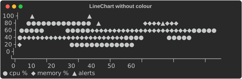
"No colour" is the console's fidelity below Rich: no
colour system, NO_COLOR, or no_color(true). Series::marker('#') picks
a series' marker; .charset(Charset::Blocks) asks for markers even with
colour.
ASCII
Charset picks the glyphs: Blocks, Braille or Ascii. The default,
Auto, is blocks for sparklines and bars and Braille for line charts. An
ASCII-only console (its encoding is not UTF-8, or its fidelity is Ascii)
always gets Ascii, whatever the chart asks for, and its output holds no
character above U+007F:
fn show_ascii(console: &Console) {
    // An ASCII-only console, or `.charset(Charset::Ascii)`.
    let ascii = Console::builder()
        .width(64)
        .color_system(None)
        .ascii_only(true)
        .build();
    let out = [
        ascii.render_to_string(&Sparkline::new(REQUESTS).min_max(true)),
        ascii.render_to_string(
            &BarChart::new()
                .bar("api", 412.0)
                .bar("web", 268.5)
                .bar_width(20),
        ),
        ascii.render_to_string(&traffic().height(6)),
    ];
    console.print(&Text::new(out.concat().trim_end()));
}
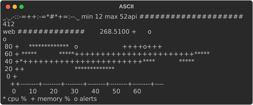
| Chart | ASCII |
|---|---|
Sparkline |
the ramp _.-:=+*#, lowest to highest |
BarChart, Histogram |
# for a cell, = for half a cell |
LineChart |
*, +, o, x, . per series; axes drawn with -, + and a vertical bar |
Gauge, BulletChart |
# and = for the bar, . and : for the bands, a vertical bar for the target |
Heatmap |
ten shades, .:-=+*#%@, and ? for a missing value |
StatusMatrix |
each state's ASCII symbol: + pass, X fail, - skip, ~ flaky |
KpiCard |
a border of +, - and vertical bars, ^ and v for the delta, the status's ASCII symbol |
Timeline |
# and = for ranges, * for milestones, ~ where a gap is cut |
Chart, Canvas |
# for the block markers, * for the others; axes and legends of -, + and vertical bars |
FillGauge, LineGauge |
# and = for the bar; - for the line |
Labels with characters above U+007F are written with ? in their place, as
fidelity::ascii_text does.
ratatui-style charts and canvases
LineChart decides its own scales, labels and legend. For a chart laid
out exactly as ratatui's Chart (so a ported app looks the same) or one
whose every part you set, use Chart:
use rich_ext::chart::{Axis, AxisScale, Chart, Dataset, GraphType, Labels, Marker};

let cpu = Dataset::new([(0.0, 0.0), (5.0, 4.0), (10.0, 1.0)])
    .name("cpu")
    .graph_type(GraphType::Line)
    .marker(Marker::Ascii('*'));
let chart = Chart::new(vec![cpu])
    .x_axis(Axis::default().bounds(0.0, 10.0).title("t").labels(Labels::Auto(3)))
    .y_axis(Axis::default().bounds(0.0, 4.0).title("%").labels(Labels::Auto(3)))
    .hidden_legend_fraction(0.5, 0.5)
    .height(8);
Axis:- bounds (or the data's extent);
- a title and its style;
- labels:
None(no axis line),Auto(n),Valuesat given values,Textspread evenly, orMarkupspread evenly with styles of their own ("[bold]0[/]", as ratatui's labels of styled spans); labels_align(HorizontalAlign::..), ratatui'slabels_alignment: the y labels' alignment in their column, and how the first x label sits against the y axis line;- a scale:
LinearorLog, where log labels fall on powers of ten; - a style;
grid([..]): lines across the plot at those values (the x axis's up the plot, the y axis's along it), drawn under the datasets in.grid_style(..)(else the axis's style) with.grid_marker(..)(else the chart's.marker(..), else the first dataset's, else Braille, so a grid before the first data looks as it will after). WithLayering::PerDataseteach line is a layer of its own, the y axis's first, so the traces break the grid where they cross it, and the x lines the y lines, as scope-tui's reference lines, drawn as datasets, break.
An axis with an empty Values list draws its line and takes no room
for labels; with Labels::None it draws no line either, as a ratatui
axis without labels (scope-tui's) does.
- Dataset:
- points;
- a name for the legend;
- a graph type: Scatter, Line, Bar (a line down to zero), or
Area (a line with the area between it and .fill_to(y) filled,
0 by default; ratatui's fill_to_y);
- a marker: Braille (2×4 dots a cell), Octant (2×4, solid),
Sextant (2×3), Quadrant (2×2), HalfBlock, Bar (▄), Block,
Dot, or Ascii(c);
- a style.
Datasets with the same marker share the dots of a cell, which takes the
later one's style; .layering(Layering::PerDataset) draws each dataset
over the ones before, as ratatui 0.29 does, so a cell a later dataset
draws in shows only its dots (where scope-tui's reference lines break
under the trace). A line, bar or area segment with an end outside the
bounds is clipped at them; .out_of_bounds(OutOfBounds::Drop) leaves it
out, as ratatui 0.29 does.
- The chart's own style, .style(".."), is ratatui's Chart::style:
it goes under every cell (a background fills the chart) and the legend's
box takes it. .style("none") is a ratatui chart with no style: the
terminal's colours, the legend's box too (.legend_unstyled() says that
by name).
- The legend is a box in a corner (LegendPosition). It hides itself
when it would cover more than hidden_legend_fraction of the plot. Its
box takes the chart's style, or else the x axis's, unless
.legend_style("..") gives it one of its own, and it clears the plot
under it; .legend_clear(false) leaves what the datasets drew there,
unstyled around the names, as ratatui does.
- The layout is ratatui's:
- the y labels sit left of a │ line and the x labels under a ─ line,
meeting at └;
- the y title sits at the top of the plot, and the x title at the right
of its last row;
- a short or narrow chart gives up parts in ratatui's order.
- The height is the height it is given, as ratatui's fills its area,
or .height(n); printed with no height, 15 rows.
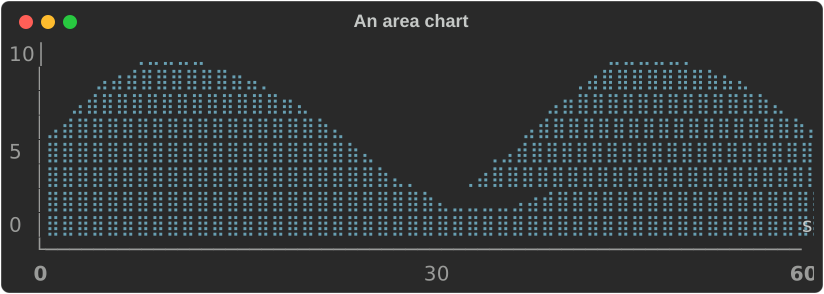
An area chart, its end labels in bold and its y labels centred:
fn show_ratatui_area(console: &Console) {
    let wave: Vec<(f64, f64)> = (0..=60)
        .map(|i| (i as f64, (i as f64 / 6.0).sin() * 4.0 + 5.0))
        .collect();
    let chart = Chart::new(vec![
        Dataset::new(wave)
            .name("load")
            .graph_type(GraphType::Area)
            .fill_to(0.0)
            .marker(Marker::Braille)
            .style("cyan"),
    ])
    .x_axis(
        Axis::default()
            .bounds(0.0, 60.0)
            .title("s")
            .labels(Labels::Markup(vec![
                "[bold]0[/]".into(),
                "30".into(),
                "[bold]60[/]".into(),
            ])),
    )
    .y_axis(
        Axis::default()
            .bounds(0.0, 10.0)
            .labels(Labels::Values(vec![0.0, 5.0, 10.0]))
            .labels_align(HorizontalAlign::Center),
    )
    .height(10);
    console.print(&chart);
}
Stacked areas
.stacked(true) puts each area dataset on top of the ones before it, so
the top edge is the running total and each band is one dataset:
fn show_areas(console: &Console) {
    let layer = |name: &str, values: [f64; 8]| {
        let points = values.into_iter().enumerate().map(|(i, v)| (i as f64, v));
        Dataset::new(points)
            .name(name)
            .graph_type(GraphType::Area)
            .marker(Marker::HalfBlock)
    };
    let chart = Chart::new(vec![
        layer("api", [12.0, 18.0, 25.0, 31.0, 28.0, 22.0, 35.0, 30.0]),
        layer("web", [8.0, 10.0, 14.0, 12.0, 18.0, 20.0, 16.0, 14.0]),
        layer("cron", [2.0, 2.0, 6.0, 2.0, 2.0, 8.0, 2.0, 2.0]),
    ])
    .x_axis(Axis::default().title("hour").labels(Labels::Auto(4)))
    .y_axis(Axis::default().labels(Labels::Auto(3)))
    .stacked(true)
    .height(12);
    console.print(&chart);
}
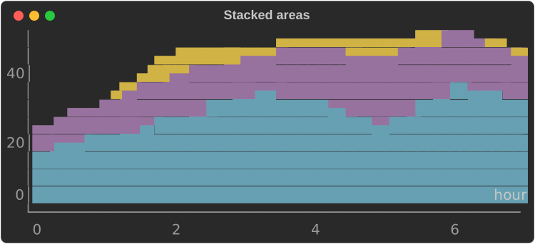
- The axes fit the totals; a linear y axis without bounds runs from the
fill level (the first area's
.fill_to(..), 0 by default). - Every stacked area fills down to that level, the top one drawn first, so
each band shows in its own style. Without colour, give each its own
marker (
Marker::Ascii('#'),Marker::Ascii('+')) to tell them apart. - Datasets that share x values stack exactly; between another area's points the one below is followed along its line. Lines, points and bars in the same chart are drawn as they are, over the areas.
- The legend and the accessible text keep each dataset's own values; the
description's first line ends
areas stacked.
Canvas draws shapes in world coordinates, as ratatui's Canvas does:
use rich_ext::chart::{Canvas, Marker};

let canvas = Canvas::new()
    .x_bounds(-1.0, 1.0)
    .y_bounds(-1.0, 1.0)
    .height(10)
    .marker(Marker::Braille)
    .paint(|p| {
        p.circle(0.0, 0.0, 0.8, "cyan");
        p.line(-1.0, -1.0, 1.0, 1.0, "red");
        p.layer();
        p.print(-0.2, 0.0, "hi", "bold");
    });
points, point, line, polyline, rect, circle, area and
print are clipped to the bounds; layer() starts a layer drawn over the
ones before, and text is drawn last. Both are renderables: print them, put
them in a table or a panel, or show them in an
intuiTUIve app with
renderable(move || chart(...)), which fills its node and draws again when
the signals it reads change.
What the canvas adds to ratatui's, and what it shares:
- A world map:
p.map(MapResolution::Low, style)draws the world's coastlines in longitude (x, -180 to 180) and latitude (y, -90 to 90); narrower bounds show a region.Lowis Natural Earth's 1:110m coastlines, simplified to about 1,200 points;Highits 1:50m ones, to about 5,000 points, with more islands. The lines are joined, so the coasts stay whole at any size. - Markers:
Quadrant(2×2 a cell),Sextant(2×3),Octant(2×4) andBar(▄), with the others. Quadrants are in every terminal font; sextants need one with Symbols for Legacy Computing (Unicode 13) and octants one with its supplement (Unicode 16). A font without them shows boxes, so choose them for terminals you know. An ASCII console gets#. - A background:
.background("on #101828")styles the cells nothing drew in and goes under what is drawn; a plain colour is taken as the background. - Shapes of your own: implement
Shape(fn draw(&self, painter: &mut CanvasPainter)) and draw it withp.shape(&it): a wireframe, a sprite, a gauge of your own.
fn show_map(console: &Console) {
    let cities = [(-0.1, 51.5), (139.7, 35.7), (-74.0, 40.7), (151.2, -33.9)];
    let world = Canvas::new()
        .x_bounds(-180.0, 180.0)
        .y_bounds(-90.0, 90.0)
        .height(18)
        .background("on #101828")
        .paint(|p| {
            p.map(MapResolution::High, "#3b8f5a");
            p.layer();
            for pair in cities.windows(2) {
                let ((x1, y1), (x2, y2)) = (pair[0], pair[1]);
                p.line(x1, y1, x2, y2, "yellow");
            }
            p.marker(Marker::Quadrant);
            for (x, y) in cities {
                p.point(x, y, "bold red");
            }
            p.print(-165.0, -45.0, "Natural Earth", "grey50");
        });
    console.print(&world);
}
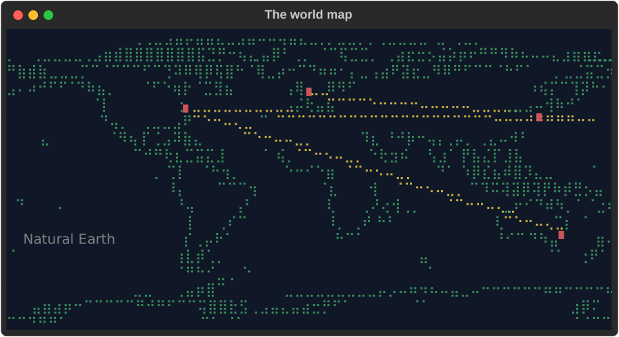
The map's data is our own, made from
Natural Earth's public-domain
coastlines by scripts/world_map.py, which simplifies them and writes the
two small files (about 5 KB and 22 KB) the crate includes. Made with
Natural Earth.
Gauges
FillGauge is ratatui's Gauge and LineGauge its LineGauge:
fn show_ratatui_gauges(console: &Console) {
    // ratatui's `Gauge`: it fills its area, the label on the middle row.
    console.print(
        &FillGauge::new(0.42)
            .label("42.00%")
            .style("magenta on grey15 italic bold")
            .unicode(true)
            .height(3),
    );
    // ratatui's `LineGauge`, in three looks.
    console.print(
        &LineGauge::new(0.42)
            .label("Downloading: 42%")
            .filled_style(tailwind::SKY.c400)
            .unfilled_style(tailwind::SLATE.c700)
            .line(LineSet::Thick),
    );
    console.print(&LineGauge::new(0.7).symbols('▰', '▱').filled_style("green"));
    console.print(&LineGauge::new(0.2).line(LineSet::Double));
}
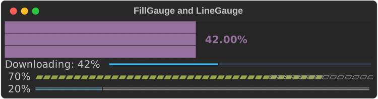
FillGauge::new(ratio)(or::percent(p)) fills the width and height it is given, left to right: whole cells, or eighths at the edge with.unicode(true). The label sits centred on the middle row, the percentage (42%) without one; over the filled part its colours are swapped, so it reads on the bar..style(..)is ratatui'sgauge_style: the foreground colours the bar, the background the rest..height(n)fixes its height; printed on its own, it is one row.LineGauge::new(ratio)writes the label (42%by default), a space, then a line to the edge:.line(LineSet::Thin | Thick | Double)or.symbols('▰', '▱'), the part up to the ratio in.filled_style(..)and the rest in.unfilled_style(..).- Both default to the theme keys
chart.gauge.filledandchart.gauge.unfilled. On an ASCII console the bar is#(=for a half) and the line-.
Level meters and spectrograms
Two charts for sound, after a DAW's meters and cava's or Audacity's spectrogram:
use std::time::{Duration, Instant};
use rich_ext::chart::{AxisScale, LevelMeter, MeterScale, PeakHold, Spectrogram};

// A peak meter in decibels, its peak held for a second.
let mut hold = PeakHold::new(Duration::from_secs(1));
let held = hold.update(peak, Instant::now());
let meter = LevelMeter::new(rms)
    .peak(peak)
    .held(held)
    .scale(MeterScale::Decibels { floor: -60.0 })
    .label("L")
    .readout(true);

// A waterfall: the newest spectrum at the top, 40 kept.
let mut waterfall = Spectrogram::new(40)
    .resolution(rate / n as f64)
    .scale(AxisScale::Log)
    .bounds(20.0, 20_000.0);
waterfall.push(spectrum.iter().map(|(_, m)| 20.0 * m.log10()));
LevelMeter::new(level)is a bar that fills to the level in eighths of a cell, then a─track to its end, with.label(..)before it and.readout(true)after (0.42, or-12.3 dB, at a fixed width so the bar keeps its place). Its cells arechart.ok(green) up to 70% of the bar,chart.warning(yellow) to 90% andchart.critical(red) past it (.bands(warning, critical))..peak(p)and.held(h)put a│mark at each.MeterScale::Linear(0 to 1 or.range(..)) orDecibels { floor }: amplitudes drawn by their decibels, from the floor to 0 dB..orientation(Orientation::Vertical)stands it up, filling the height it is given from the bottom.PeakHold::new(hold)keeps a peak:update(peak, now)returns the highest peak of the lasthold, then drops to the peak then (.fall(per_second)lets it fall at a rate instead).Spectrogram::new(rows)keeps the newestrowsspectra;push(levels)adds one at the top. Each row is the levels as aHeatmap's shades (░▒▓█, ASCII.:-=+*#%@, and thechart.heat.Ncolours, cold to hot), scaled between the lowest and highest kept or.range(..). The bins are spread across the width, evenly or by their logarithm (.scale(AxisScale::Log), each octave as wide);.resolution(hz)and.bounds(low, high)say which frequencies the width covers. A column over several bins shows the loudest. It fills the height it is given.
Bar spectra and persistence
cava's bars and an analogue scope's phosphor:
use rich_ext::chart::{BarSpectrum, Chart, Layering, Persistence};
use rich_ext::dsp::{bands, Falloff};

// 24 bands from 50 Hz to 10 kHz, falling under gravity, mirrored.
let mut falloff = Falloff::gravity(0.02);
let levels = falloff.update(&bands(&spectrum, 24, 50.0, 10_000.0)).to_vec();
let bars = BarSpectrum::new(levels).mirror(true).bar_width(2);

// The last eight traces, each older one fainter.
let fading = Persistence::new(traces).style("#33ff66").fade(0.2);
let scope = Chart::new(fading.datasets()).layering(Layering::PerDataset);
BarSpectrum::new(bands)draws each band as a column from the bottom, its top in eighths of a cell (#s to the whole cell in ASCII), scaled to the loudest band or.range(max),.bar_width(n)cells wide and.gap(n)apart, centred..mirror(true)draws the bands twice, the low ones in the middle;BarSpectrum::stereo(left, right)puts a channel on each side. Too narrow, it drops the gaps, then narrows the bars, then lets bands share a column. It fills the height it is given.Persistence::new(frames)takes the last frames of a trace, oldest first, and makes them datasets in the frame's style, each older one's colour faded towards.background(..)(black) down to.fade(floor)of it. Draw them withLayering::PerDataset, so the newest is on top.
intuiTUIve draws these as nodes with its viz feature: meter(level,
peak).hold(d), spectrogram(|| rows) and bar_spectrum(|| bands); see
intuiTUIve's levels.
In tables and panels
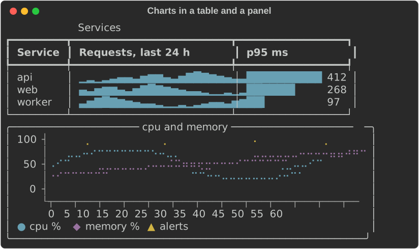
A sparkline measures to one cell per value and a bar chart to its label, bar
and value, so they fit table columns. A line chart takes the width it is
given, or .width(n):
fn show_table(console: &Console) {
    let mut table = Table::new().title("Services");
    table.add_column("Service");
    table.add_column("Requests, last 24 h");
    table.add_column("p95 ms");
    for (name, offset, p95) in [("api", 0, 412.0), ("web", 6, 268.0), ("worker", 12, 97.0)] {
        let values = REQUESTS.iter().cycle().skip(offset).take(24).copied();
        table.add_row_cells(vec![
            Cell::Markup(name.into()),
            Cell::Renderable(Arc::new(Sparkline::new(values))),
            Cell::Renderable(Arc::new(
                BarChart::new()
                    .bar("", p95)
                    .max(500.0)
                    .bar_width(12)
                    .format(ValueFormat::Fixed(0)),
            )),
        ]);
    }
    console.print(&table);
    let panel = Panel::new(Box::new(traffic().width(56).height(5)))
        .title("cpu and memory")
        .expand(false);
    console.print(&panel);
}
Gauges and bullet charts
A Gauge shows one value against a range. .target(t) draws a │ across
the bar where the target is, and each Band is a threshold: the band runs
up to its value, the bar takes the band's style while the value is in it,
and the band's name is written after the value.
fn show_gauges(console: &Console) {
    let cpu = Gauge::new("cpu", 72.0)
        .range(0.0, 100.0)
        .target(80.0)
        .band(Band::new(60.0, "ok").style("chart.ok"))
        .band(Band::new(85.0, "high").style("chart.warning"))
        .band(Band::new(100.0, "critical").style("chart.critical"))
        .unit("%");
    // One line: label, bar, value and the band the value is in.
    console.print(&cpu.clone().bar_width(24));
    // Full width: a scale under the bar and a legend.
    console.print(&cpu.full_width(true));
    console.print(&Text::new(""));
    // Several gauges with their columns aligned.
    let quarter = BulletChart::new()
        .gauge(Gauge::new("revenue", 270.0).range(0.0, 300.0).target(250.0))
        .gauge(Gauge::new("profit", 22.5).range(0.0, 30.0).target(26.0))
        .gauge(
            Gauge::new("new customers", 1650.0)
                .range(0.0, 2000.0)
                .target(1800.0)
                .band(Band::new(1400.0, "poor").style("chart.critical"))
                .band(Band::new(1700.0, "fair").style("chart.warning"))
                .band(Band::new(2000.0, "good").style("chart.ok")),
        )
        .bar_width(30);
    console.print(&quarter);
}
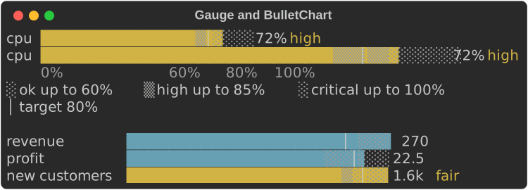
- The bar fills with eighth-cell blocks (
█▉▊▋▌▍▎▏), half-cell Braille, or#and a half=in ASCII. The rest of the track is shaded by band, alternating░and▒(.and:), so each band's extent shows without colour. - The scale runs from 0 (or the smallest of the value, the target and the
bands) to the largest of them;
.range(min, max)fixes it. - The compact form is one line, with a bar of
.bar_width(n)cells (20 by default)..full_width(true)fills the width and adds a scale line (the bounds, the target and the band edges, each at its cell) and a legend (░ ok up to 60% │ target 80%). - Given less width the bar shrinks to 4 cells, then the band's name goes, then the value, then the label is cut.
BulletChartstacks gauges with their labels, bars, values and band names in aligned columns. Each keeps its own scale, target and bands.
Heatmaps
A Heatmap is a grid of values, a row per label and a column per header,
each cell a shade from the lowest value to the highest:
fn show_heatmap(console: &Console) {
    let hours: Vec<String> = (0..24).map(|h| format!("{h:02}")).collect();
    let mut map = Heatmap::new().columns(hours);
    for (day, name) in ["mon", "tue", "wed", "thu", "fri", "sat", "sun"]
        .into_iter()
        .enumerate()
    {
        let weekend = if day >= 5 { 0.4 } else { 1.0 };
        let load = (0..24).map(|h| {
            let peak = (-((h as f64 - 14.0).powi(2)) / 30.0).exp();
            (peak * 900.0 * weekend + 40.0 * day as f64).round()
        });
        map = map.row(name, load);
    }
    console.print(&map);
    // In ASCII: ten shades, so it reads in black and white.
    let ascii = Console::builder()
        .width(60)
        .color_system(None)
        .ascii_only(true)
        .build();
    console.print(&Text::new(ascii.render_to_string(&map).trim_end()));
}
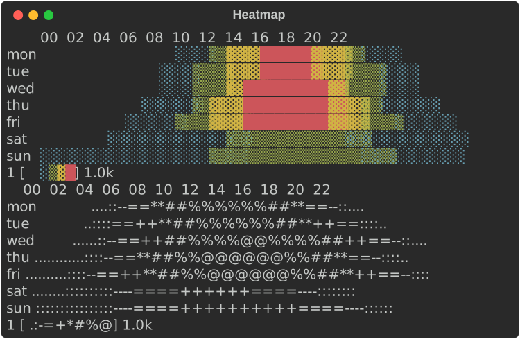
- Values are scaled into equal steps: five in blocks (
░▒▓█), ten in ASCII (.:-=+*#%@). The shade is the value, so the grid reads in black and white; with colour each step also takes achart.heat.Nstyle, cold to hot..range(min, max)fixes the scale. - A NaN or infinite value is drawn
·(?in ASCII), never as a low value, and the legend says so. - Each value is
.cell_width(n)cells wide (2 by default). A header is written at its column's first cell when it fits with a space after the one before, so with narrow cells every second or third header shows. - Given less width the cells narrow to one, then the row labels are cut, then neighbouring columns are merged, each showing the mean of its values, so every value still counts.
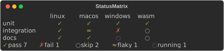
Status matrices
A StatusMatrix is rows and columns of states, such as a test suite
across platforms. Each state is a symbol and a colour, never colour
alone, and the legend counts the cells in each:
fn show_matrix(console: &Console) {
    let matrix = StatusMatrix::new()
        // Your own state: a name, a symbol, an ASCII symbol and a style.
        .state(State::new("running", '◌', 'o', "chart.state.unknown"))
        .columns(["linux", "macos", "windows", "wasm"])
        .row("unit", ["pass", "pass", "pass", "pass"])
        .row("integration", ["pass", "flaky", "fail", "skip"])
        .row("docs", ["pass", "pass", "running", "skip"]);
    console.print(&matrix);
}
| State | Symbol | ASCII | Theme key |
|---|---|---|---|
pass |
✓ |
+ |
chart.state.pass |
fail |
✗ |
X |
chart.state.fail |
skip |
○ |
- |
chart.state.skip |
flaky |
≈ |
~ |
chart.state.flaky |
State::new(name, symbol, ascii, style)adds a state, or replaces a built-in one with the same name. A symbol must take one cell; a wide one is replaced by its ASCII form.- A name with no state is drawn
?inchart.state.unknownand named in the legend as it is. A row shorter than the headers leaves its last cells blank. - Columns are as wide as their widest header. Given less width the headers are cut (and left out below three cells), then the row labels, then the gaps; columns that still do not fit are left off the right.
.counts()returns how many cells are in each state.
KPI cards
A KpiCard is one key number: a label, the value, its change, an optional
sparkline and an optional Status:
fn show_cards(console: &Console) {
    let cards = vec![
        KpiCard::new("Requests", 12_400.0)
            .unit("/s")
            .previous(11_430.0)
            .caption("last week")
            .trend(trend(0.0))
            .status(Status::Ok),
        KpiCard::new("Errors", 42.0)
            .delta(-14.0)
            .higher_is_better(false)
            .caption("per hour")
            .trend(trend(4.0))
            .status(Status::Warning),
        KpiCard::new("Latency", 412.0)
            .unit(" ms")
            .previous(260.0)
            .higher_is_better(false)
            .trend(trend(8.0))
            .status(Status::Critical),
    ];
    let cells = cards
        .into_iter()
        .map(|card| Cell::Renderable(Arc::new(card.width(24))))
        .collect();
    console.print(&Columns::from_cells(cells));
}
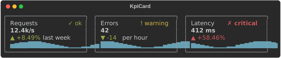
- The change is an arrow and a signed number:
▲ +8.49%,▼ -14,= 0(^,vand=in ASCII)..delta(d)gives an amount,.delta_percent(p)a percentage and.previous(v)the percentage change fromv. A change that is NaN or too large for anf64reads= -: no sign, and the flat arrow. It is styledchart.delta.goodorchart.delta.badby whether the change is for the better:.higher_is_better(false)for errors, latency and costs. The arrow and the sign carry the direction without colour. Status::Ok,Warning,CriticalandUnknownare a symbol and a word (✓ ok,! warning,✗ critical,? unknown) inchart.ok,chart.warning,chart.criticalorchart.unknown.- A card measures to its content, so cards sit side by side in
Columnsor a table..width(n)fixes its width, border included, and.expand(true)fills what it is given, as in aLayout. Cards with the same parts have the same height, so a row of them lines up. .border(false)leaves the border out; below 5 cells it goes anyway.
Timelines and Gantt strips
A Timeline puts labelled ranges on a numeric scale, such as the steps of
a build in seconds. Ranges with the same row label share a row:
fn show_timeline(console: &Console) {
    let build = Timeline::new()
        .span("fetch", 0.0, 4.0)
        .span("compile", 4.0, 26.0)
        // Overlapping ranges on one row are stacked.
        .span("test", 12.0, 30.0)
        .span("test", 20.0, 34.0)
        .span("package", 34.0, 39.0)
        .milestone("ship", 40.0)
        .unit("s")
        .width(60);
    console.print(&build);
    console.print(&Text::new(""));
    // Ten minutes idle between two short bursts: the gap is cut out.
    let jobs = Timeline::new()
        .span("worker 1", 0.0, 3.0)
        .span("worker 1", 3.0, 5.0)
        .span("worker 2", 2.0, 6.0)
        .span("worker 1", 600.0, 604.0)
        .span("worker 2", 602.0, 610.0)
        .milestone("deploy", 611.0)
        .unit("s")
        .width(60);
    console.print(&jobs);
}
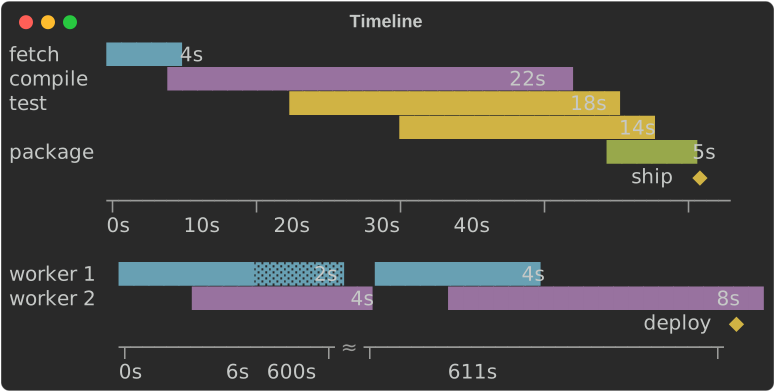
- Ranges on one row that overlap are stacked onto extra lines, so none
hides another. A range that starts where the one before it on its line
ends is drawn
▓instead of█(=instead of#), so both show. - A range covers every column whose centre value is inside it, and at least
one. Its length is written after it when there is room
(
.durations(false)leaves them out), so it reads without the axis. .milestone(label, at)marks a point with◆(*) on a line under the ranges, its label beside it.- The axis labels sit on evenly spaced columns and name each column's exact
value, as on a line chart;
.unit("s")writes a unit after every value. The scale is plain numbers: pass seconds (or any unit) asf64. - Compression: when the range is wider than the plot, so that the
shortest range would get less than a column, idle gaps are cut out when
they are longer than both four times the shortest range and three
columns' worth of the uncut scale. Each cut takes three columns with
≈(~) on the axis, and each stretch is labelled at its start and end..compress(false)keeps the scale linear;.range(min, max)fixes it. - It fills the width given, or
.width(n). Given less, the row labels are cut so the plot keeps 8 columns.
A dashboard
Cards, a matrix and a timeline in a Layout, rebuilt and passed to
Live::update on every tick, make a live dashboard. The
kpi_dashboard
example runs one; this is a frame of a smaller one:
fn dashboard() -> Layout {
    let card = |c: KpiCard| Layout::with_renderable(Box::new(c.expand(true)));
    let mut cards = Layout::new().size(6);
    cards.split_row(vec![
        card(
            KpiCard::new("Requests", 1240.0)
                .unit("/s")
                .previous(1180.0)
                .trend(trend(0.0)),
        ),
        card(
            KpiCard::new("Errors", 7.0)
                .delta(2.0)
                .higher_is_better(false)
                .trend(trend(5.0))
                .status(Status::Warning),
        ),
    ]);
    let checks = StatusMatrix::new()
        .columns(["eu", "us", "ap"])
        .row("api", ["pass", "pass", "flaky"])
        .row("worker", ["pass", "fail", "pass"]);
    let deploy = Timeline::new()
        .span("build", 0.0, 18.0)
        .span("test", 12.0, 34.0)
        .span("rollout", 36.0, 52.0)
        .milestone("live", 60.0)
        .unit("s");
    let mut root = Layout::new();
    root.split_column(vec![
        cards,
        Layout::with_renderable(Box::new(Panel::new(Box::new(checks)).title("checks"))).size(6),
        Layout::with_renderable(Box::new(Panel::new(Box::new(deploy)).title("deploy"))),
    ]);
    root
}
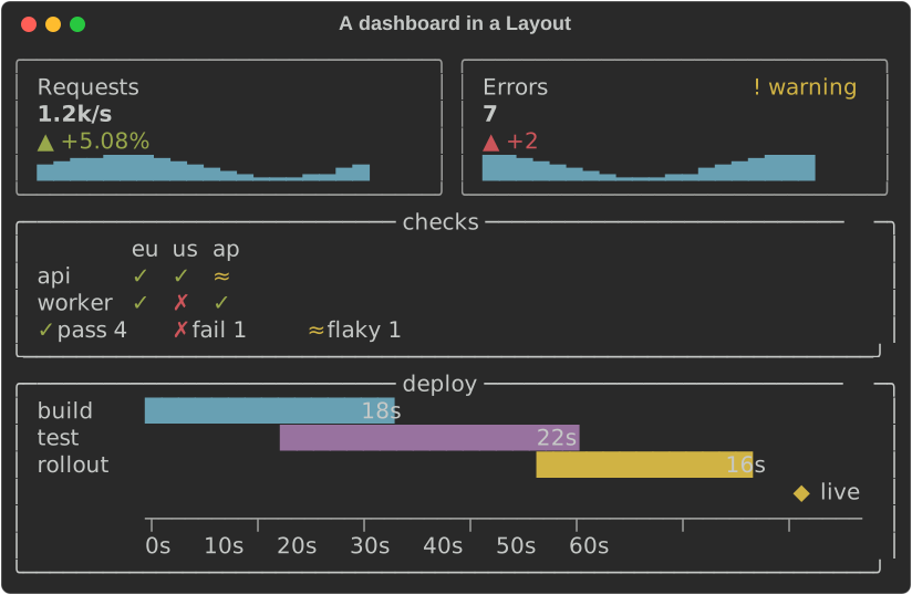
Cards take .expand(true) to fill their region. The layout fills the
console's height, so give Live a console with a fixed .height(n) or let
it take the terminal's.
Distributions
Distribution::new(values) sums a set of values up on one line: a
box-and-whisker strip, then the numbers. A DistributionSet stacks several
on one scale:
fn show_distribution(console: &Console) {
    // One set of values: a box-and-whisker strip, then the numbers.
    let latency = Distribution::new(latencies())
        .label("latency")
        .format(ValueFormat::Fixed(0));
    console.print(&latency);
    // Several on one scale, their numbers in columns.
    let set = DistributionSet::new()
        .push(
            Distribution::new(latencies())
                .label("api")
                .format(ValueFormat::Fixed(0)),
        )
        .push(
            Distribution::new(latencies().iter().map(|v| v * 0.6 + 15.0))
                .label("web")
                .format(ValueFormat::Fixed(0)),
        )
        .push(
            Distribution::new(latencies().iter().map(|v| v * 1.3))
                .label("worker")
                .format(ValueFormat::Fixed(0)),
        );
    console.print(&set);
}

- The strip runs from the smallest value to the largest:
├and┤at the ends,─whiskers, a shaded box▒from the first quartile to the third, the median█, and the 95th percentile a┼on the whisker when it has a cell of its own. In ASCII:|,-,=,#and+. The glyphs carry it, so it reads without colour. With colour, the box and the median arechart.bar(or.style(..)) and the whiskerschart.axis. - The numbers are the count
n,min,p25,p50(the median),p75,p95,maxandmean, in.format(..)with.unit(..)after each value. NaN and infinite values are left out and counted (2 ignored). - Quantiles are numpy's default, linear interpolation (Hyndman and
Fan's type 7): for
nsorted values, theqquantile sits at position(n - 1) q, between the two values either side of it. One value is every quantile. No values drawno dataandn 0. .summary()returns the numbers as aSummary.Summary::of(values)andquantile(&sorted, q)compute them without drawing.- The strip is
.strip_width(n)cells (20 by default). Given less width it shrinks to 8 cells, then the numbers shorten tomin,p50andmax, then they go, then the label is cut..range(min, max)fixes the scale, and.numbers(false)leaves the numbers out. DistributionSetdraws every row on one scale: the smallest to the largest value of them all, or.range(..). Labels, strips and numbers sit in aligned columns, and the scale's two ends are written under the strips..shared_scale(false)gives each row its own scale.
Small multiples
SmallMultiples::new([(title, chart), …]) lays charts out in a grid, each
under its title, all on one value scale, so they compare at a glance:
fn show_multiples(console: &Console) {
    // A sparkline per service on one scale: the busiest stands out.
    let services = [
        ("api", 1.0),
        ("web", 0.6),
        ("worker", 0.3),
        ("search", 0.8),
        ("auth", 0.45),
        ("cron", 0.1),
    ];
    let grid = SmallMultiples::new(
        services.map(|(name, share)| (name, Sparkline::new(REQUESTS.map(|v| v * share)))),
    );
    console.print(&grid);
    // Line charts in three columns, with one legend under them.
    let region = |phase: f64| {
        let wave = move |i: usize| ((i as f64 + phase) / 4.0).sin();
        LineChart::new()
            .series(Series::from_values(
                "p50",
                (0..24).map(|i| 40.0 + 15.0 * wave(i)),
            ))
            .series(Series::from_values(
                "p99",
                (0..24).map(|i| 70.0 + 25.0 * wave(i)),
            ))
            .height(5)
    };
    let regions = [
        ("eu", region(0.0)),
        ("us", region(3.0)),
        ("ap", region(6.0)),
    ];
    console.print(&SmallMultiples::new(regions).columns(3));
}
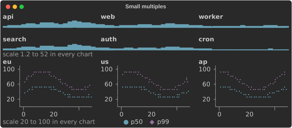
- Columns:
.columns(n), or as many as fit cells of at least.min_cell_width(n)(24 by default) with.gap(n)cells between them (2 by default). That is one column at 40 cells, three at 80 and four at 120, never more than there are charts. Every cell is as wide; what is left over stays at the right. Charts fill the grid row by row. - One scale: a
Facetis a chart whose value scale can be shared: aSparkline(its heights), aBarChart(its bars' lengths, from zero), aLineChartor aChart(the y axis). Each converts with.into(). The grid fixes every chart's scale to the range of them all, so a taller bar is a larger value whichever chart it is in. When a chart has axis labels the range is rounded out to round numbers..range(min, max)fixes it, and.shared_scale(false)leaves each chart its own. - One note under the grid says the scale (
scale 0 to 60 in every
  chart
) and holds the one legend: the line charts' series, whose own legends are left out..note(false)leaves it out. - Height:
.height(rows)makes each chart that many rows. Without it, a grid given a height (aLayoutregion, an intuiTUIve node) shares it among its rows of charts, less the titles, the gaps and the note. Printed on its own, each chart keeps its own height. - Titles are
chart.title(bold), cut to the cell. A blank line separates the rows of charts.
Accessible text
Every chart implements rich_ext::a11y::AccessibleText: a few short lines
of plain words that say what the chart shows, for a screen reader, a log or
a test. There are no glyphs or box lines in it, and it reads the same
whatever the width or the console:
fn show_accessible(console: &Console) {
    // What each chart says to a screen reader: plain words, no glyphs.
    let gauge = Gauge::new("cpu", 72.0)
        .range(0.0, 100.0)
        .target(80.0)
        .band(Band::new(60.0, "ok"))
        .band(Band::new(85.0, "high"))
        .unit("%");
    let texts = [
        Sparkline::new(REQUESTS).accessible_text(80),
        traffic().accessible_text(80),
        gauge.accessible_text(80),
        Histogram::new(latencies()).bins(8).accessible_text(80),
    ];
    console.print(&Text::new(texts.join("\n\n")));
}
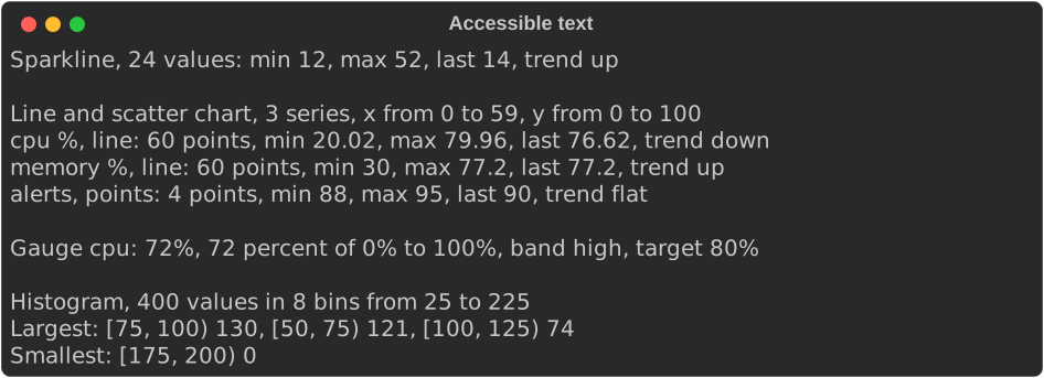
The first line says what the chart is, how much it holds and the ranges of its axes. The lines after it give the key values:
| Chart | First line | Then |
|---|---|---|
Sparkline |
Sparkline, 24 values: min 12, max 52, last 14, trend up, with the gaps (1 missing) and a threshold (4 above 40) |
|
BarChart |
Bar chart, 4 bars in 2 groups, values from 2 to 4, 1 without a value |
every bar, up to six; else Largest: the three largest and Smallest: the smallest |
Histogram |
Histogram, 400 values in 8 bins from 25 to 225 |
each bin's count, up to six bins; else the largest and the smallest |
LineChart |
Line chart, 3 series, x from 0 to 59, y from 0 to 100 |
a line per series: its name, line or points, then 60 points, min 20.02, max 79.96, last 76.62, trend down |
Chart |
Chart, 2 datasets, x (t) from 0 to 10, y (%) from 0 to 4, and log scale for a log axis |
a line per dataset, as a line chart's |
Gauge, BulletChart |
Gauge cpu: 72%, 72 percent of 0% to 100%, band high, target 80% |
a bullet chart: a line per gauge |
FillGauge, LineGauge |
Gauge 50/100 GB: 50 percent |
|
Heatmap |
Heatmap, 2 rows by 4 columns, values from 0 to 9, 1 missing |
Highest 9 at api, wed; lowest 0 at web, mon |
StatusMatrix |
Status matrix, 3 rows by 3 columns: 4 pass, 2 fail, 1 skip |
the cells of each state but pass and skip: fail: unit on windows, docs on macos |
KpiCard |
KPI Errors: 42, down 25% vs yesterday, better, status warning |
its sparkline's text |
Timeline |
Timeline, 3 rows, 3 ranges, 1 milestone, from 0s to 52s |
each range (compile from 4s to 31.5s, 27.5s), twenty at most, and each milestone |
Canvas |
Canvas, x from -180 to 180, y from -90 to 90: a world map, 4 points, 3 lines |
Text: what it printed |
Distribution |
Distribution latency: 400 values, min 27, p25 64, median 81, …, mean 87 |
|
DistributionSet |
Distributions, 3 on a shared scale from 27 to 287 |
each distribution's line |
SmallMultiples |
Small multiples, 6 charts on a shared scale from 1.2 to 52 |
each chart's title and text |
- Values are written in the chart's own format, counts with thousands separators.
- A series' trend is the least-squares line through its finite
points:
upordownwhen it rises or falls by at least a tenth of the values' range across the series,flatotherwise. A hump that ends where it began is flat. - In an intuiTUIve app, draw a chart with
described(move || ..)instead ofrenderable(..). It looks the same, and its accessible name is the chart's text, its lines joined with.. The accessibility tree, linear mode and a screen reader read the description, and read it again when the data changes..label("CPU")goes first:CPU: Line chart, …. - From Python:
rs_rich.chart.describe(chart), orrs_rich.ext.a11y.accessible_text(chart).
From the shell: rich chart
rich chart draws data from a file, a URL or stdin with these charts, so a
shell pipeline can end in a picture. It reads CSV and TSV (the dialect
sniffed as rich --csv sniffs it), JSON (an array of records, of numbers or
of rows, or an object of columns), JSON Lines, or whitespace-separated
numbers.
rich chart sales.csv                                  # every numeric column as a line
rich chart sales.csv --kind bar --x month --y api     # a bar per row, labelled
rich chart sales.csv --kind heatmap                   # rows by series, as shades
rich chart sales.csv --kind pie --y api               # one series as slices
rich chart sales.csv --kind stacked                   # a bar per row, series as parts
seq 1 20 | rich chart --kind spark                    # numbers piped in
rich chart metrics.json --kind scatter --x t --y p50 --y p99
| Option | Meaning |
|---|---|
--kind spark\|bar\|line\|scatter\|heatmap\|pie\|stacked |
What to draw; line by default. A pie draws one series: name it with --y when there are several |
--x COLUMN |
The positions (line, scatter: numbers) or labels (bar, heatmap, pie, stacked). Default: the row number; for labels, the first column that is not all numbers |
--y COLUMN |
A series; repeat for several. Default: every numeric column but --x |
--width N |
The width to draw in |
Columns go by header or by 1-based number, so a CSV without a header works
too (its columns are 1, 2, ...). An empty cell or a JSON null is a gap.
A column that is not there, or a value that is not a number, is refused with
exit code 4 and a message naming the row (counted from 1, after the header)
and the column:
$ rich chart sales.csv --y mobile
rich: no column "mobile"; the columns are "month", "api", "web"
$ rich chart sales.csv --x month
rich: row 1, column "month": "Jan" is not a number (a line or scatter chart's --x is a position; --kind bar takes labels)
$ rich chart sales.csv --kind bar --y api --width 50
Jan ███████████████████████▌                 30
Feb █████████████████████████████████        42
Mar ███████████████████████████▌             35
Apr ████████████████████████████████████████ 51
May █████████████████████████████████████▋   48
The recording shows it in a terminal.
Colours: palettes and helpers
rich_ext::palette has the colours charts and apps are often drawn in, as
ratatui's style::palette and its palette feature have:
palette::tailwind: Tailwind CSS's 22 palettes (SLATEtoROSE), each with eleven shades fromc50toc950, andtailwind::ALLwith their names.palette::material: Material Design's 19 palettes,c50toc900, and the accentsa100toa700of the 16 that have them.- Each shade is a
#rrggbbstring, so it goes straight into markup (format!("[on {}]", SLATE.c900)), a style or a theme. - Colours from numbers, each a truecolor
rich::Color:hsl(h, s, l)andhsv(h, s, v), with the hue in degrees;oklab(l, a, b); andokhsv(h, s, v), HSV whose hues are evenly spaced to the eye and whose value looks the same lightness at every hue, so a swatch of it has no bright bands. blend(a, b, t)mixes two colours, andgradient(&stops, t)picks a colour along several spaced evenly.style_from_color_name(name)reads a colour named as ratatui reads one (DarkGray,light red,#FF8800,208) as rich's name for the same terminal colour (bright_black,bright_red,#ff8800,color(208)), orNone: a ported app's colour options, without ratatui. rs-rich-ratatui re-exports it.
fn show_palette(console: &Console) {
    // Tailwind's shades, as markup.
    let mut strip = String::new();
    for (_, palette) in tailwind::ALL.iter().skip(5).step_by(2) {
        for shade in palette.shades() {
            strip.push_str(&format!("[on {shade}] [/]"));
        }
        strip.push(' ');
    }
    console.print(&Text::from_markup(&strip).unwrap());
    // An Okhsv swatch in half blocks: the hue across, the value down.
    let swatch = Canvas::new()
        .x_bounds(0.0, 59.0)
        .y_bounds(0.0, 3.0)
        .width(60)
        .height(2)
        .marker(Marker::HalfBlock)
        .paint(|p| {
            for y in 0..4 {
                for x in 0..60 {
                    let colour = okhsv(f64::from(x) * 6.0, 0.9, 1.0 - f64::from(y) / 6.0);
                    let hex = colour.get_truecolor().map(|t| t.hex()).unwrap_or_default();
                    p.point(f64::from(x), f64::from(3 - y), &hex);
                }
            }
        });
    console.print(&swatch);
}

Credit: Tailwind CSS's palette is MIT licensed (Tailwind Labs); Material Design's colours come from Material Design Lite, Apache License 2.0 (Google); Oklab and Okhsv are Björn Ottosson's, and the conversions are our own code for his published formulas.
Gradient text
rich_ext::gradient::GradientText colours a Text along two or more
colours (gradient(&stops, t) for each character), across, down or
corner to corner:
fn show_gradient(console: &Console) {
    let sunset = [
        tailwind::AMBER.c400,
        tailwind::ROSE.c500,
        tailwind::VIOLET.c600,
    ]
    .map(|hex| Color::parse(hex).expect("a colour"));
    let title = Text::from_markup("[bold]rs-rich: rich, in Rust[/]").expect("markup");
    console.print(&GradientText::new(title, sunset.clone()));
    let block = Text::new("one gradient\nfrom the top\nto the bottom");
    console.print(&GradientText::new(block, sunset.clone()).direction(GradientDirection::Vertical));
    let banner = Text::new("  behind the text  ");
    console.print(&GradientText::new(banner, sunset).background(true));
}
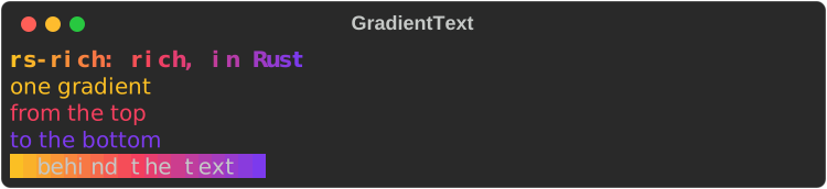
- The text is laid out as it would be on its own (wrapped, justified, its
bold and italic kept); then each character takes the colour at its
column across the widest line (
GradientDirection::Horizontal, the default), its line (Vertical) or both (Diagonal). - The gradient replaces the text's own colour;
.background(true)paints the background instead. - It degrades by colour system: each colour is the nearest the console
has, so 256 colours show steps and 16 colours a few bands, and
neighbours that come out the same are written as one run. Without colour
(
NO_COLOR, a pipe) the text is drawn as it is. Its accessible text is the text's own words.
QR codes
rich_ext::qr::QrCode (the qr feature) encodes text or bytes and draws
the code with half blocks, two modules a cell, so it is square and a phone
can read it off the terminal:
fn show_qr(console: &Console) {
    let code = QrCode::with_error_correction(
        "https://github.com/buchochelliq-labs/rs-rich-cli",
        ErrorCorrection::Medium,
    )
    .expect("fits a QR code");
    // Scanners manage with two modules of quiet zone; the spec asks for four.
    console.print(&code.quiet_zone(2));
}
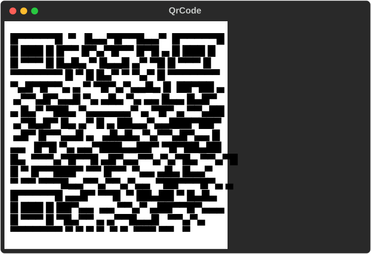
QrCode::new(text)usesErrorCorrection::Medium;QrCode::with_error_correction(text, level)takesLow(about 7% of the code can be lost),Medium(15%),Quartile(25%) orHigh(30%), and uses a higher level when it fits the same size of code.QrCode::from_bytes(bytes, level)encodes bytes. Data too long for the largest code (version 40) is aQrError::TooLong.- With colour every cell is painted, the dark modules
#000000and the light ones#ffffff(.colours(dark, light)changes them), so the code reads on a dark or a light terminal. - Without colour the glyphs draw the light modules, so on a dark
terminal the code reads dark on light;
.invert(true)draws the dark ones, for a light terminal. - ASCII (
Charset::Ascii, or an ASCII-only console) draws a module as##or two spaces (painted spaces with colour), twice as tall. - The quiet zone is 4 modules, as the specification asks;
.quiet_zone(2)is smaller and scanners manage. Given less width, the quiet zone narrows to a module; a code that still does not fit is replaced byQR code needs N columns, as a cut code cannot be read. .size(),.version(),.error_correction()and.module(x, y)read the code back. The accessible text names the version, the size, the error correction and what it encodes.
The encoder is Project Nayuki's
qrcodegen (MIT, no dependencies):
one file, lighter to build than qrcode, whose image and SVG renderers
this crate has no use for.
All of them together, from the same example:
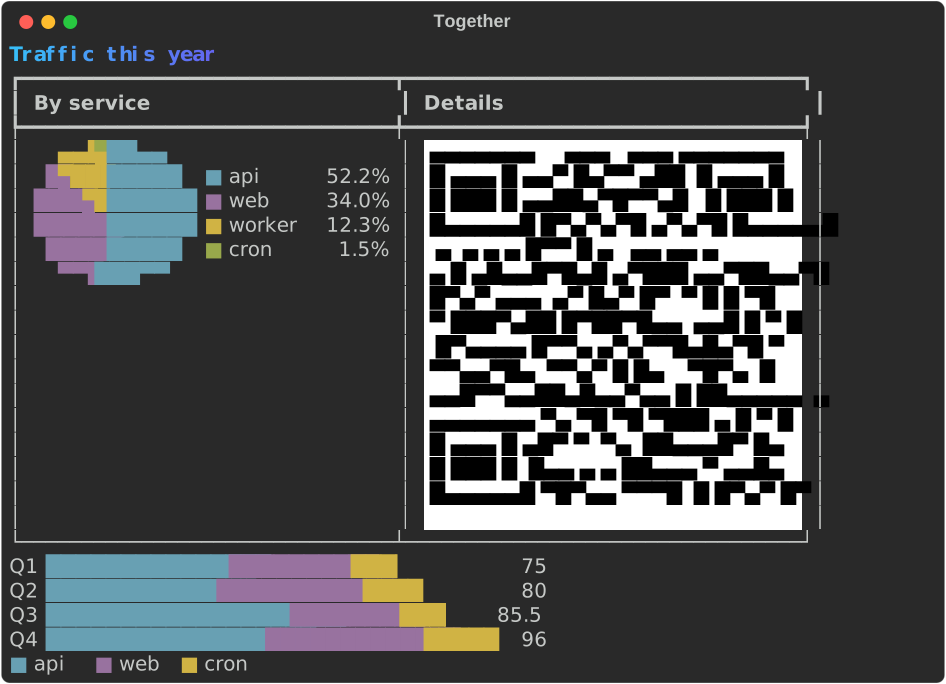
The code
fn show_together(console: &Console) {
    let blue = [tailwind::SKY.c400, tailwind::INDIGO.c500].map(|c| Color::parse(c).unwrap());
    let title = Text::from_markup("[bold]Traffic this year[/]").unwrap();
    console.print(&GradientText::new(title, blue));
    let code = QrCode::new("https://example.com/traffic")
        .unwrap()
        .quiet_zone(1);
    let mut row = Table::new();
    row.add_column("By service");
    row.add_column("Details");
    row.add_row_cells(vec![
        Cell::Renderable(Arc::new(traffic().height(6))),
        Cell::Renderable(Arc::new(code)),
    ]);
    console.print(&row);
    console.print(&quarters().bar_width(36));
}
The shared pieces
| Type | What it does |
|---|---|
Scale |
A linear scale. Scale::from_values skips NaN and infinities and never has an empty range: when every value is v the range is twice as wide as v with v in the middle (0..1 for 0), and no values gives 0..1. .nice(n) widens to round bounds; .ticks(n) gives about n round values inside it; .normalize(v) maps to 0..1 |
ValueFormat |
Compact (950, 0.25, 1.2k, 3.4M, 1.0e15 from a thousand trillion) or Fixed(decimals) (at most ValueFormat::MAX_DECIMALS, 17; more are capped) |
Status |
A health level for a KpiCard: a symbol, a word and a theme key |
State |
A state of a StatusMatrix cell: a name, a symbol, an ASCII symbol and a style |
Band, Span, Milestone |
A gauge's threshold band; a timeline's range and point |
Charset |
Auto, Blocks, Braille, Ascii |
DotCanvas |
The Braille canvas the line chart draws on: set dots, draw lines, read cells |
Direction, Levels |
A sparkline's way (LeftToRight, RightToLeft) and block set (Nine, Three) |
BarGroup |
Bars with a label, set apart from the others, or .stacked() into one bar |
Slice |
A pie's slice: a label, a value and an optional style |
Marker, Shape, MapResolution |
How a canvas marks what it draws; a shape of your own; the map's detail |
LineSet |
A line gauge's glyphs: Thin, Thick, Double |
Summary, quantile |
A distribution's numbers (Summary::of(values)), and one quantile of sorted values, interpolated linearly |
Facet |
A chart a SmallMultiples grid can hold and put on its shared scale: Sparkline, BarChart, LineChart or Chart |
Theme keys:
| Key | Default | Used for |
|---|---|---|
chart.axis |
bright_black |
Axes and ticks |
chart.label, chart.value |
none | Labels, tick labels and values |
chart.bar |
cyan |
Bars |
chart.negative |
magenta |
Bars below zero |
chart.spark |
cyan |
Sparklines |
chart.over |
bold red |
Sparkline values above the threshold |
chart.min, chart.max |
blue, bold green |
Sparkline extremes |
chart.series.1 … .5 |
cyan, magenta, yellow, green, blue |
Series, by position (they cycle); timeline rows; pie slices; stacked parts |
chart.track |
bright_black |
A gauge's track and band shades |
chart.target |
bold |
A gauge's target marker |
chart.gauge.filled, chart.gauge.unfilled |
cyan, bright_black |
A FillGauge's bar and the rest; a LineGauge's two parts |
chart.ok, chart.warning, chart.critical, chart.unknown |
green, yellow, bold red, bright_black |
Status, and bands that name them |
chart.delta.good, chart.delta.bad, chart.delta.flat |
green, red, bright_black |
A KPI card's change |
chart.kpi.label, chart.kpi.value, chart.kpi.border |
none, bold, bright_black |
A KPI card |
chart.heat.1 … .5 |
blue, cyan, green, yellow, red |
Heatmap steps, cold to hot |
chart.state.pass, .fail, .skip, .flaky, .unknown |
green, bold red, bright_black, yellow, magenta |
Status matrix states |
chart.milestone |
bold yellow |
Timeline milestones |
chart.title |
bold |
Small multiples' titles |